38 excel pivot chart rotate axis labels
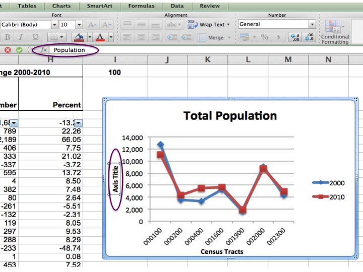
How to Add Axis Titles in a Microsoft Excel Chart - How-To Geek Select your chart and then head to the Chart Design tab that displays. Click the Add Chart Element drop-down arrow and move your cursor to Axis Titles. In the pop-out menu, select "Primary Horizontal," "Primary Vertical," or both. If you're using Excel on Windows, you can also use the Chart Elements icon on the right of the chart. Excel Paste And Transpose Shortcut - Automate Excel Paste & Transpose This Excel Shortcut pastes and transposes. PC Shorcut:Ctrl+ALT+V>E>Enter Mac Shorcut:Ctrl+⌘+V>⌘+E>Return Remember This Shortcut: Ctrl + V is the usual command to Paste. Simply add Alt for Paste Special and use E for Transpose. Alernatively you can use Alt > E > S > E . Remember, Alt is the command to activate…
Rotate charts in Excel - spin bar, column, pie and line charts 09/07/2014 · If the chart you need to rotate in Excel displays Horizontal and Vertical axes, you can quickly reverse the order of the categories or values plotted along those axes. Additionally, in 3-D charts that have a depth axis, you can flip the plotting order of data series so that large 3-D columns do not block smaller ones. You can also reposition the Legend on your pie or column …

Excel pivot chart rotate axis labels
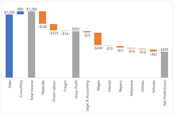
How to Overlay Charts in Microsoft Excel - How-To Geek In the Change Chart Type window, select Combo on the left and Custom Combination on the right. Create your chart: If you don't have a chart set up yet, select your data and go to the Insert tab. In the Charts section of the ribbon, click the drop-down arrow for Insert Combo Chart and select "Create Custom Combo Chart." Excel Charts – Spilled Graphics With the MOD and SEQUENCE functions it´s possible to rotate a pie chart. When done properly it can offer the possibility to be the “Gateway chart”, meaning it can be used as an entry point, allowing you to communicate a simple fact that you can use as a reference point, but then connect it to more detailed data. Many thanks to Jorge ... Excel Waterfall Chart: How to Create One That Doesn't Suck - Zebra BI In this case the only viable option would be to break the vertical axis and have the totals start at some value larger than 0. Let's say 35,000. This highlights individual contributions, but risks guiding unaware readers to false conclusions about the data. You can again resort to using tutorials and templates:
Excel pivot chart rotate axis labels. How to Show Percentage in Pie Chart in Excel? - GeeksforGeeks 29/06/2021 · To add data labels, select the chart and then click on the “+” button in the top right corner of the pie chart and check the Data Labels button. Pie Chart It can be observed that the pie chart contains the value in the labels but our aim is … How to Add Two Data Labels in Excel Chart (with Easy Steps) Table of Contents hide. Download Practice Workbook. 4 Quick Steps to Add Two Data Labels in Excel Chart. Step 1: Create a Chart to Represent Data. Step 2: Add 1st Data Label in Excel Chart. Step 3: Apply 2nd Data Label in Excel Chart. Step 4: Format Data Labels to Show Two Data Labels. Things to Remember. How to Format Data Labels in Excel (with Easy Steps) Then, in the Select Data Source dialog box, click on the Edit option from the Horizontal Axis Labels. In the Axis Labels dialog box, select column B as the Axis label range. Then, click on OK. Finally, click on OK in the Source Data Source dialog box. Finally, we get the following chart. See the screenshot. Data Labels in Excel Pivot Chart (Detailed Analysis) 7 Suitable Examples with Data Labels in Excel Pivot Chart Considering All Factors 1. Adding Data Labels in Pivot Chart 2. Set Cell Values as Data Labels 3. Showing Percentages as Data Labels 4. Changing Appearance of Pivot Chart Labels 5. Changing Background of Data Labels 6. Dynamic Pivot Chart Data Labels with Slicers 7.
Chart.Axes method (Excel) | Microsoft Docs This example adds an axis label to the category axis on Chart1. VB Copy With Charts ("Chart1").Axes (xlCategory) .HasTitle = True .AxisTitle.Text = "July Sales" End With This example turns off major gridlines for the category axis on Chart1. VB Copy Charts ("Chart1").Axes (xlCategory).HasMajorGridlines = False How to Create and Customize a Waterfall Chart in Microsoft Excel Select the chart and use the buttons on the right (Excel on Windows) to adjust Chart Elements like labels and the legend, or Chart Styles to pick a theme or color scheme. Select the chart and go to the Chart Design tab. Then, use the tools in the ribbon to select a different layout, change the colors, pick a new style, or adjust your data ... Home - Automate Excel Add Axis Labels: Add Secondary Axis: Change Chart Series Name: Change Horizontal Axis Values: Create Chart in a Cell: Graph an Equation or Function: Overlay Two Graphs: Plot Multiple Lines: Rotate Pie Chart: Switch X and Y Axis: Insert Textbox: Move Chart to New Sheet: Move Horizontal Axis to Bottom: Move Vertical Axis to Left: Remove Gridlines ... chandoo.org › wp › show-months-years-in-chartsShow Months & Years in Charts without Cluttering » Chandoo ... Nov 17, 2010 · So you can just have Product Group & Product Name in 2 columns and when you make a chart, excel groups the labels in axis. 2. Further reduce clutter by unchecking Multi Level Category Labels option. You can make the chart even more crispier by removing lines separating month names. To do this select the axis, press CTRL + 1 (opens format dialog ...
How to Create a Workflow in Excel (3 Simple Methods) You don't need to insert a new shape again. Select the shape and press CTRL+C to copy it. Then press CTRL+V to paste it there. Now you can select and drag the shapes to align them properly. Use CTRL+Select to select multiple shapes. Then select Shape Format >> Arrange >> Align. Adjusting the Order of Items in a Chart Legend (Microsoft Excel) This area details the data series being plotted. You can select one of the entries and use the up and down arrows (just to the right of the Remove button) to adjust the order in which the entries are plotted. When you click OK, the chart is replotted and the legend updated to reflect the plotting order. spilledgraphics.com › excel-charts-with-dynamic-arraysExcel Charts – Spilled Graphics Combining Dynamic Arrays with the Pareto Principle 80/20, but with a different touch: a “vertical Pareto” for improved readability on the category labels. In data visualization aiming for legibility is key. Many thanks to Jon Peltier (The Da Vinci of Excel Charts) for blogging 11 years ago about building vertical Paretos. How to Rotate Axis Labels in Excel (With Example) - Statology The following chart will automatically appear: By default, Excel makes each label on the x-axis horizontal. However, this causes the labels to overlap in some areas and makes it difficult to read. Step 3: Rotate Axis Labels. In this step, we will rotate the axis labels to make them easier to read. To do so, double click any of the values on the ...
How to Change Horizontal Axis Labels in Excel 2010 - Solve Your Tech
How to group (two-level) axis labels in a chart in Excel? The Pivot Chart tool is so powerful that it can help you to create a chart with one kind of labels grouped by another kind of labels in a two-lever axis easily in Excel. You can do as follows: 1. Create a Pivot Chart with selecting the source data, and: (1) In Excel 2007 and 2010, clicking the PivotTable > PivotChart in the Tables group on the ...
32 How To Label Vertical Axis In Excel - Labels Database 2020
Creating a horizontal bar chart off of averages [SOLVED] Re: Creating a horizontal bar chart off of averages 1. Click Right anywhere in the PT Average left hand scale (column B) and select Sort Highest to lowest. Then refresh the PT 2. It's always advisable to tidy up your original data and eliminate #NA altogether.

Excel Horizontal Axis Labels Not Showing Up - retpalion
Excel Chart: Multi-level Lables. Hello experts! I have a bar chart that uses a multi-level category, similar to the example below. To save space in the Y axis labelling area, I'd like to have car manufacturers names on top of each bar while retaining the group names (=country) in the Y axis with a bar for each manufacturer.

Best Excel Tutorial - 3 axis chart
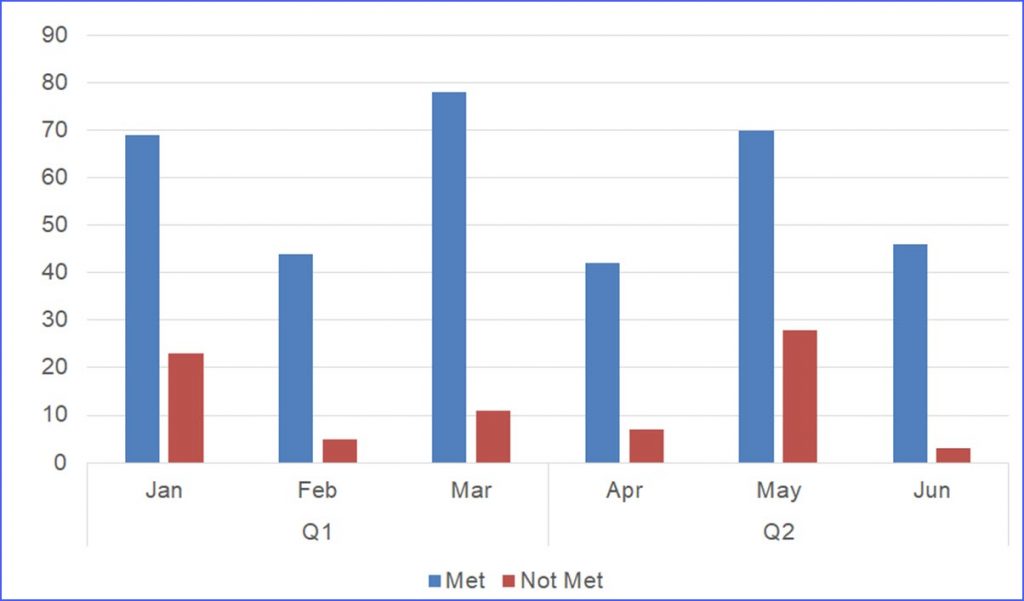
Two-Level Axis Labels (Microsoft Excel) - ExcelTips (ribbon) Just select your data table, including all the headings in the first two rows, then create your table. Excel automatically recognizes that you have two rows being used for the X-axis labels, and formats the chart correctly.
31 How To Label Vertical Axis In Excel
› documents › excelHow to group (two-level) axis labels in a chart in Excel? The Pivot Chart tool is so powerful that it can help you to create a chart with one kind of labels grouped by another kind of labels in a two-lever axis easily in Excel. You can do as follows: 1. Create a Pivot Chart with selecting the source data, and: (1) In Excel 2007 and 2010, clicking the PivotTable > PivotChart in the Tables group on the ...

How to Resize a Table - ExcelNotes
Can you change the text alignment of a Data Table in a Pivot ... You want the labels "Junk Data #" to be rotated 90 degrees. Right click on one of the data labels, to select the whole block Select "Format Axis" option to display the Format Axis Pane In the Format Axis pane > Axis Options > Size & Properties (3rd hieroglyphic icon) > Text Direction > pick which way you want to rotate it. Report abuse

Overlapping Bar Chart Google Sheets - Free Table Bar Chart
Matplotlib X-axis Label - Python Guides We import the matplotlib.pyplot package in the example above. The next step is to define data and create graphs. plt.xlabel () method is used to create an x-axis label, with the fontweight parameter we turn the label bold. plt.xlabel (fontweight='bold') Read: Matplotlib subplot tutorial.
37 How To Label Vertical Axis In Excel - Labels Design Ideas 2021
How to Make a Pie Chart with Multiple Data in Excel (2 Ways) - ExcelDemy After following the steps of how to create pivot tables, we can get the following output. Now, we will use the following steps to make a Pie Chart. Steps: First, select the data set and go to the Insert tab from the ribbon. After that, click on the Pivot Chart from the Charts group. Now, select Pivot Chart from the drop-down.
36 How To Label The Axis In Excel - Modern Labels Ideas 2021
Show Months & Years in Charts without Cluttering - Chandoo.org 17/11/2010 · I've got a pivot chart with months of data and all I had to do was right-click the x axis and then select "format axis", under "Axis Options" there's a check-box that says "Multi-level Category Labels". The chart I was able to do this on was a pivotchart however so maybe it wouldn't be that easy for a non-pivotchart. Anyway, love the site. Keep ...

Rotate charts in Excel 2010-2013 – spin bar, column, pie and line charts
How to Change the X-Axis in Excel - Alphr Open the Excel file with the chart you want to adjust. Right-click the X-axis in the chart you want to change. That will allow you to edit the X-axis specifically. Then, click on Select Data. Next ...

Multilevel Pivot Table Excel | I Decoration Ideas
How to create a chart in Excel from multiple sheets - Ablebits.com 05/11/2015 · Click on the chart you've just created to activate the Chart Tools tabs on the Excel ribbon, go to the Design tab (Chart Design in Excel 365), and click the Select Data button. Or, click the Chart Filters button on the right of the graph, and then click the Select Data… link at the bottom. In the Select Data Source window, click the Add button.
Text Labels on a Vertical Column Chart in Excel - Peltier Tech Blog
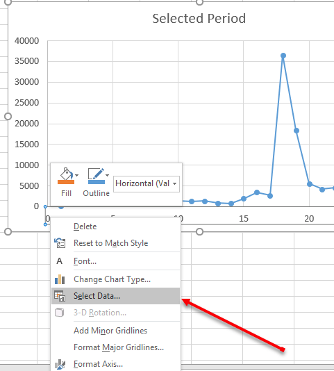
Pivot Chart Settings | MyExcelOnline Switch Row/Column - You can use this option to change the way data is plotted in PivotCharts. You can swap the data over the axis with this quickly and revert back when needed. Select Data - You can change the data source of your Pivot Chart using this option. Change Chart Type - There are a lot of different chart types that you can change quickly.
How to Create a Chart with the Axis having Two Categories - ExcelNotes
How to make and use Pivot Table in Excel - Ablebits.com 2. Create a Pivot Table. Select any cell in the source data table, and then go to the Insert tab > Tables group > PivotTable. This will open the Create PivotTable window. Make sure the correct table or range of cells is highlighted in the Table/Range field. Then choose the target location for your Excel Pivot Table:

34 What Is A Category Label In Excel - Labels Design Ideas 2020
› how-to-show-percentage-inHow to Show Percentage in Pie Chart in Excel? - GeeksforGeeks Jun 29, 2021 · To add data labels, select the chart and then click on the “+” button in the top right corner of the pie chart and check the Data Labels button. Pie Chart It can be observed that the pie chart contains the value in the labels but our aim is to show the data labels in terms of percentage.

32 How To Label Vertical Axis In Excel - Labels Database 2020
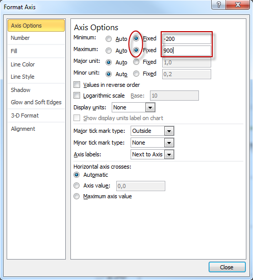
Format Chart Axis in Excel - Axis Options Right-click on the Vertical Axis of this chart and select the "Format Axis" option from the shortcut menu. This will open up the format axis pane at the right of your excel interface. Thereafter, Axis options and Text options are the two sub panes of the format axis pane. Formatting Chart Axis in Excel - Axis Options : Sub Panes
how to flip bar chart in excel - Unese.campusquotient.org
Key Features by Version - Origin Excel Like Formula Bar ... Box Chart: Connect Lines Support for Connection Types, Percentile Symbols Support Edge Thickness Control Wrap Text in Tick Labels that Contain No Spaces Transparency Support for Image Plot from Matrix Data Align Option for Multi-line Data Labeling Longer Minus Sign in Tick Labels Remove Exponential Notation Common to All Tick Labels …
31 How To Label Vertical Axis In Excel
exceljet.net › lessons › how-to-reverse-a-chart-axisExcel tutorial: How to reverse a chart axis In this video, we'll look at how to reverse the order of a chart axis. Here we have data for the top 10 islands in the Caribbean by population. Let me insert a standard column chart and let's look at how Excel plots the data. When Excel plots data in a column chart, the labels run from left to right to left.
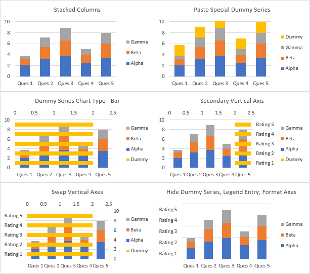
How to Create a Chart with Two-level Axis labels in Excel - Free Excel Tutorial
Axis Labels | WinForms Controls | DevExpress Documentation Select an axis in the diagram, and locate the Axis2D.CustomLabels property in the Properties window. Click its ellipsis button to invoke the Custom Axis Label Collection Editor. Click Add to create a label and set its CustomAxisLabel.AxisValue and ChartElementNamed.Name properties.
Post a Comment for "38 excel pivot chart rotate axis labels"